Chapter 0: Basics of Python
Chapter Introduction
This is a statistics course, but the opening chapter develops the Python foundations needed to work with data. A result is easier to trust when you can explain how its inputs were selected, how a function used them, and what its output means. If items[0:4], key=lambda …, **kwargs, or a KeyError looks unfamiliar, it is harder to tell whether an unexpected result comes from the data, the calculation or the code. This chapter explains those mechanics with small, runnable examples before you use them for statistical analysis.
The chapter starts with numbers and strings, then builds up to containers, control flow and functions. A few mental models connect the examples. A name is a label attached to an object, and assignment moves labels rather than copying objects. Some objects can be edited in place and some cannot: this explains why b = a behaves differently for an integer and for a list. Slices and ranges include their start and exclude their stop, from s[0:4] to range(1, 5). A function’s default argument is evaluated once when the function is defined, rather than each time it is called. Learning these rules turns surprising outputs into consequences you can explain.
Small code errors can produce plausible results without raising an exception. Check the length of a slice, trace changes to a shared list, and try a function on a small example whose output you can predict. These habits make errors visible before you use the result in a business decision.
By the end of the chapter you will be able to predict, before running, what Python prints for arithmetic that mixes integers and floats; slice any sequence — string, list or tuple — and say exactly how many elements the slice holds; explain what happens to a when you modify b after b = a, and choose between .copy() and a second name deliberately; pick the right container for a job (a tuple for a fixed record, a set for membership, a dictionary for a lookup); write if/for/while logic and compress the common case into a comprehension; define functions with defaults, *args and **kwargs, and avoid the mutable-default bug; format numbers with f-strings; and convert a crash into a value with try/except. The text-analysis guided practice example — counting the most frequent words in a paragraph of raw text — uses every one of those pieces in a dozen lines and is, structurally, the same programme as a bag-of-words sentiment score on an earnings-call transcript.
The final section explains installation and imports, numerical arrays and normal-model probabilities. Its delivery-service examples use the same parameters and units in the book, slides and adapted videos.
The chapter follows the five sections of the companion slide deck in the same order, with the same examples and the same printed numbers, so that the two can be read side by side. Each subsection gives the mechanism in prose, then a runnable cell, then an interpretation of what the cell printed. Some cells are wrapped as “predict the output”: commit to an answer on paper before you click reveal, because a prediction that turns out wrong is worth ten that turn out right. Two cells are marked “debug yourself” and contain a bug that does not raise an error — the dangerous kind. Flashcards at the end of each section are for spaced review before the exam.
How to use the numbered learning path
Follow the numbered parts in order within each section. Each part states a question and a result. Read the concept, predict the example, run it, and explain the output before attempting the check.
The 3.5-hour class selects examples, group discussion and notebook work. The complete Slides and Book support self-study.
Worked examples run automatically when the page opens or refreshes. Each cell includes required earlier imports, data and definitions under Previously introduced setup. Run Code includes that setup; Copy complete code copies the whole cell. Practice and repair cells run when you choose. Make input changes in the current cell before the operation you are testing.
Table of Contents
- Values, Numbers and Strings
- Containers and Object Identity
- Branches, Loops and Comprehensions
- Functions, Formatting and Error Handling
- Modules, NumPy and SciPy
Values, Numbers and Strings
| Part | Question |
|---|---|
| 0.1.1 Values and numerical expressions | How does Python evaluate and store a calculation? |
| 0.1.2 Booleans and comparisons | How does a comparison become a decision? |
| 0.1.3 Strings, slices and methods | How do we select and clean recorded text? |
Values and numerical expressions
Question: How does Python evaluate and store a calculation?
Result: Trace an expression, assignment and numerical type.
Begin with the definitions and assumptions; then trace the worked example.
Values and the execution model
Begin with one value and ask what its type allows. An expression combines values to produce another value; assignment, written =, binds a name to that result. For units = 10, price = 44.99 and amount = units * price, Python evaluates the multiplication before binding amount. The name is not a spreadsheet formula that recalculates automatically: changing price later does not change amount until the multiplication line runs again. == asks whether two values compare equal; it does not assign.
Each browser cell includes its required earlier definitions in a folded setup panel. In Colab, the kernel remembers names from earlier cells; restarting it clears them. Within a cell, statements execute from top to bottom. Predict an output, run the cell, change one input and explain the difference. Browser slides require no installation; the in-class notebook is completed and saved in Colab.
The slice illustration labels every character, including a visible symbol for a space. Start is inclusive and stop is exclusive. Changing the step changes which eligible positions are visited. This positional rule also applies to lists and tuples.
You already know arithmetic. What this section is about is where Python’s arithmetic differs from the calculator on your desk: a division operator that always returns a float, a second division operator that rounds down rather than toward zero, a floating-point representation in which 0.1 + 0.2 is not 0.3, a True that is secretly the integer 1, and a text type that behaves like a list you are not allowed to edit. None of these is an obscure corner of the language. Every price, return and p-value in this course is a float; every count of “up days” is a sum of booleans; every ticker and column name is a string. The differences are small, and they are exactly where the wrong number comes from.
Expressions, and the two divisions
An expression is anything Python can evaluate to a value: 1 + 2, (3 - 1) * 5 / 2, 2 ** 10. In a notebook the value of the last expression in a cell is displayed automatically; in a script, or when you want more than one value from a cell, you wrap it in print(). The arithmetic operators are the ones you expect, with two deliberate departures from calculator notation. Exponentiation is **, not ^ — in Python ^ is bitwise exclusive-or, which is a legal operation on integers and therefore fails silently rather than loudly: 2 ^ 10 is 8, not 1024. And the remainder (modulo) operator is %, so 10 % 3 is 1.
The subtler departure is division. Python 3 has two division operators. True division / always returns a float, even when the mathematical answer is a whole number: 4 / 2 is 2.0, not 2. Floor division // returns the largest integer not greater than the exact quotient; for positive operands that is the familiar “integer part”, but for negative operands it rounds toward minus infinity rather than toward zero, so -10 // 3 is -4, not -3. The remainder is defined to be consistent with the floor, so that a == (a // b) * b + a % b always holds; a consequence is that -10 % 3 is 2, and in Python the sign of a % b follows the sign of b.
Why does this matter in finance? Lot sizing. Shares on many exchanges trade in board lots of 100; shares // 100 counts the whole lots and shares % 100 is the odd lot. For a long position of 1,250 shares that gives 12 lots and 50 odd shares, and every language agrees. For a short position represented as −1,250 shares, Python’s floor gives -13 lots and an odd lot of 50, whereas a language that truncates toward zero would report −12 and −50. Neither is “wrong”, but if you split the sizing logic between Python and SQL or C and do not know which convention each one uses, the lot count on the short book is off by one.
Four expressions, four lines. Write down what each prints — paying attention to whether the second line shows 5 or 5.0 — before you reveal the output.
The four lines print 3, 5.0, 1024 and 1. The one that catches people is the second: the exact answer is the whole number five, but because the expression contains a /, the result is the float 5.0. Python never silently turns a float back into an integer, so once a / appears anywhere in a calculation, everything downstream of it is a float, and type() will tell you so.
The first line is 3.3333333333333335 — sixteen significant digits, of which the last is an artefact of binary representation that we return to below. The second is 3 -4 1: floor division of -10 by 3 is -4 because −3.33… lies between −4 and −3 and the floor is the lower of the two. The third line confirms the type rule: / produced a float, // produced an int. The lot-sizing lines print 12 50 for the long position and -13 50 for the short one — the whole-lot count on the short side is −13, not −12, and the remainder is positive because it takes the sign of the divisor.
Use / whenever the answer is a quantity (a return, a ratio, an average). Use // only when the answer is a count of whole units (lots, weeks, pages) and be explicit about the sign convention. If you find yourself writing int(a / b) to get a whole number, you are truncating toward zero — which is fine, but it is not the same as a // b for negative a, and the two will disagree exactly when it matters.
Booleans and comparisons
Question: How does a comparison become a decision?
Result: Interpret True and False and check numerical precision.
Builds on Values and numerical expressions.
int, float, bool, and what type() tells you
Python has four scalar types you will use constantly. An int is a whole number of unbounded size — 2 ** 100 is a perfectly good integer and Python will happily print all thirty-one of its digits. A float is a double-precision binary floating-point number in the IEEE 754 standard: 64 bits, of which 53 carry the significand, giving roughly 15–17 significant decimal digits. A bool is one of True or False. A str is text. The built-in function type(x) returns the type of any value, and it is the first thing to print when a calculation gives a result you did not expect.
Arithmetic between an int and a float promotes the result to float: 42 + 3.14159 is 45.14159, a float. Python never truncates in the other direction, so the danger with mixed arithmetic is not lost precision from the integer but the false confidence of thinking a value is exact when it is a float. The point at which you will feel this most is comparison. Because a float is a binary fraction, most decimal numbers cannot be represented exactly: 0.1 is stored as the nearest 53-bit binary fraction, which is 0.1000000000000000055511151231257827…, and 0.2 likewise. Their sum is the nearest representable number to the sum of the two approximations, and that turns out to be 0.30000000000000004, which is not the same double as the nearest representable number to 0.3. So 0.1 + 0.2 == 0.3 is False.
For computed quantities that should be approximately equal, choose a tolerance appropriate to the units and numerical scale. In this example abs(x - y) < 1e-9 is sufficient. math.isclose supports relative and absolute tolerances. Exact equality remains useful for labels, categories and deliberately recorded values; it is approximate arithmetic that needs care.
Booleans are the smallest surprise and the most useful one. In Python bool is a subclass of int: True behaves as 1 and False as 0 in any arithmetic context. So True + True is 2, True * 3.5 is 3.5, and — the reason you should care — sum(list_of_booleans) counts how many were True. For example, sum([True, False, True]) is 2: two of the three values are true. Dividing that count by 3 gives the fraction, 2 / 3.
The first three lines show the promotion rule: <class 'int'> 42, <class 'float'> 3.14159, and then <class 'float'> 45.14159 for the sum. The next three are the float trap in full: False, then 0.30000000000000004, then True once the comparison is made with a tolerance of one part in a billion. The last three lines are the boolean-as-integer rule: 1, then <class 'bool'> 2 — note that the type is still bool but the sum is the integer 2 — and finally 3 of 4 conditions were True, which is the idiom you will use for counting.
== on floats, is on anything but None
Two comparison habits will save you from most silent errors in this course. Use a suitable tolerance when comparing calculated floats that should be approximately equal. And never use is to compare values at all; is asks whether two names point to the same object, which is a question about memory, not about value. The only idiomatic use of is is x is None. Section 0.2 explains why.
Strings, slices and methods
Question: How do we select and clean recorded text?
Result: A correctly sliced and cleaned string with the result assigned.
Builds on Booleans and comparisons.
Strings are sequences: indexing and slicing
A string holds text, and in Python it is a sequence: an ordered collection of characters that you can index and slice with exactly the same syntax you will later use on lists and tuples.
Indexing is s[i]. Positions count from zero, so s[0] is the first character. Negative positions count from the end, so s[-1] is the last character and s[-2] the one before it; this is a convenience Python offers so that you do not have to write s[len(s) - 1]. Slicing is s[start:stop:step], and the rule to memorise is start inclusive, stop exclusive: s[0:4] gives the characters at positions 0, 1, 2 and 3, and not position 4. Any of the three parts may be omitted — s[:4] starts from the beginning, s[5:] runs to the end, s[::2] takes every second character from the start.
The half-open convention looks arbitrary until you see what it buys. For a forward slice with step 1 and valid boundaries satisfying 0 <= a <= b <= len(s), the number of elements in s[a:b] is b - a, with no +1 to remember. Two adjacent slices s[:k] and s[k:] tile the sequence exactly, with no overlap and no gap, which is precisely what you want when splitting data into a training set and a test set. And s[i:i+n] contains n elements when that many remain in the sequence, which is the shape of every rolling calculation in Chapter 1. The half-open rule lets you check a window’s intended length by subtraction.
With s = 'data Analysis', work out what s[0:4] and s[::2] are — write the characters of s with their positions 0 to 12 on paper first — and then reveal all six lines.
The string has 13 characters. s[0] is d and s[-1] is s. s[0:4] and s[:4] are both data — positions 0, 1, 2, 3, and not the space at position 4. s[5:] is Analysis, the eight characters from position 5 to the end. s[::2] is dt nlss: positions 0, 2, 4, 6, 8, 10 and 12, which are d, t, the space, n, l, s, s. The common wrong answer for s[::2] is aaAayi — the characters at the odd positions — which is what you get if you assume the step starts after the first character rather than at it. It does not: a slice always begins at start, which defaults to 0.
A last observation that will matter in Chapter 1: slicing past the end does not raise an error. s[5:100] is still Analysis; Python clamps the stop to the length. That is convenient, and it is also why a window that runs off the end of a price list shrinks silently rather than failing. Printing len() of the slice is the only defence.
Objects have methods, and strings are immutable
Everything in Python is an object, and every object carries functions that belong to it, called methods. You invoke a method with a dot: object.method(arguments). A string has dozens — .strip() removes whitespace from both ends, .upper() and .lower() change case, .replace(old, new) substitutes text, .split(sep) cuts one string into a list of strings at every occurrence of the separator. Even an integer has methods: (10).bit_length() tells you that 10 needs 4 bits in binary. You can discover what an object can do with the same dot-syntax: in a notebook, type the name, a dot, and press Tab.
The method to remember from this section is .split(). It turns one string into a list of strings, and it is the first step of every text-processing task, including the guided practice example at the end of the chapter: a paragraph becomes a list of words by paragraph.split(), which with no argument splits on any run of whitespace, including newlines. The reverse operation is the string method .join(), called on the separator: ", ".join(["a", "b", "c"]) is "a, b, c".
The property that separates strings from lists is that a string is immutable: once created, it cannot be changed. There is no s[0] = "D" — that is a TypeError. It follows that every string method that appears to modify the string in fact returns a new string and leaves the original untouched. s.upper() on its own does nothing visible: it computes an upper-case copy, and because you did not assign the copy to anything, it is discarded. To keep the result you must write s = s.upper(), which creates the new string and rebinds the name s to it. A common text-cleaning mistake is to call a string method and forget to keep its returned value.
The first four lines are hello, world, HELLO, WORLD, hello, Python and ['data', 'science', '101']; note that .upper() and .replace() left the leading and trailing spaces alone because only .strip() removes them. 10 .bit_length() is 4, since 10 in binary is 1010. Then the immutability demonstration: after a bare s.upper() the string is still ' hello, world ' — repr() shows the quotes and the spaces that print() would hide — and only after s = s.upper() does it become ' HELLO, WORLD '. The last line chains two methods: .strip() returns a new string, and .upper() is called on that, giving 'HELLO, WORLD'. Chaining works because the first method returns a string on which the next string method can be called.
An immutable value can be shared freely. If two variables point to the same string, neither can change it under the other’s feet, so you never need to copy a string defensively. Immutability is also what allows strings (and tuples) to be dictionary entry names, which Section 0.2 explains. The price is that “modifying” a string means building a new one — negligible for a ticker, noticeable for a million-character transcript, which is why text pipelines build a list of pieces and .join() them once at the end.
10 / 3 is 3.3333333333333335 (a float, always — / returns a float even when the answer is whole). 10 // 3 is 3 (an int). -10 // 3 is -4, not -3: floor division rounds toward minus infinity, so −3.33 floors to −4.
Neither 0.1 nor 0.2 is exactly representable as a binary fraction; the sum of their nearest doubles is 0.30000000000000004, which is not the double nearest 0.3. Compare with a tolerance: abs(x - y) < 1e-9, or math.isclose(x, y). Never == on floats.
It shows ' hello ', unchanged. Strings are immutable: .upper() returns a new string, and because the result was not assigned it was discarded. To keep it write s = s.upper().
Containers and Object Identity
| Part | Question |
|---|---|
| 0.2.1 Lists, identity and copies | Can two names refer to the same mutable object? |
| 0.2.2 Tuples and sets | Do we need fixed order or unique membership? |
| 0.2.3 Dictionaries and container checks | How do names connect to stored values? |
Lists, identity and copies
Question: Can two names refer to the same mutable object?
Result: Trace an edit through an alias and through an independent copy.
Begin with the definitions and assumptions; then trace the worked example.
Choosing a container by its purpose
A list holds an ordered collection that you can edit. A tuple holds a fixed sequence: individual elements cannot be replaced, although a mutable object inside a tuple can itself change. A set supports membership and uniqueness without positional access. A dictionary maps names to values and is useful for named policy choices. A dictionary preserves insertion order, but a lookup such as policy["capacity"] uses the name rather than a row position.
Choose the structure before memorising its methods. Ask whether order matters, whether you need unique members, whether entries need names and whether the collection will change. For policy = {"percentile": 0.75, "capacity": 100}, changing policy["percentile"] leaves policy["capacity"] at 100. These are separate names, and the mapping makes the distinction explicit.
The arrows distinguish names from objects. In alias mode both names refer to the same list, so appending through either name changes the shared object. Copy mode creates an independent outer list. This is a shallow copy; it is sufficient for these integer elements, but it does not recursively copy nested mutable containers.
Python has four built-in ways to hold many values. A list is an ordered, editable sequence; a tuple is an ordered sequence that cannot be edited; a set is an unordered collection of unique values; a dictionary is a mapping from names to values. Two questions classify them. Does it have positions? Lists and tuples do, so you can index and slice them; sets and dictionaries do not, and bag[0] is an error. Can it be changed after creation? Lists, sets and dictionaries can — they are mutable; tuples cannot. The second question is the important one, because mutability is the property behind the trap that bites every analyst once: what happens to a when you change b.
Lists: ordered, mutable, mixed types
A list is written with square brackets, may contain values of different types, and supports the same indexing and slicing as a string: nums[1:-1] is everything except the first and last elements. What a list adds is a family of methods that edit it in place: .append(x) adds one element at the end, .insert(i, x) puts x at position i and shifts the rest along, .pop() removes and returns the last element (or .pop(i) for position i), .remove(x) deletes the first occurrence of a value, .sort() reorders. None of these returns a new list; they modify the one you called them on and return None (except .pop, which returns the removed item). This is the opposite convention from strings, and mixing the two up produces the classic nums = nums.append(50), after which nums is None.
nums[1:-1] is [20, 30] — positions 1 up to but not including the last. After .append(50) the list is [10, 20, 30, 40, 50]. .insert(1, 15) makes it [10, 15, 20, 30, 40, 50], and .pop() removes the trailing 50, so the third line prints [10, 15, 20, 30, 40] removed: 50. The fourth line — 10 40 [15, 20] — is indexing and slicing again, identical to the string case. The last line shows three operations that you will use on every list: len() is 5, the membership test 30 in nums is True, and nums.index(30) is 3, the position of the first 30.
The aliasing trap: names and objects
Here is the mental model that explains everything else in this section. In Python a variable is not a box that holds a value; it is a name — a label — attached to an object that lives somewhere in memory. The assignment nums = [10, 20, 30, 40] creates a list object and attaches the label nums to it. The assignment alias = nums does not create a second list. It attaches a second label, alias, to the same object. There is still exactly one list, with two names. Assignment never copies.
Now consider alias.append(50). The method is called on the object that alias points to, and it mutates that object. Because nums points to the very same object, nums “sees” the 50 as well — not because Python did anything to nums, but because there was never anything else for nums to be. Two names, one list. If you wanted alias to be independent, you had to ask for a copy: nums.copy(), or equivalently list(nums) or the full slice nums[:], each of which builds a new list object with the same contents.
Why does the same assignment feel harmless for integers? Because integers are immutable. After a = 5; b = a, both names point to the same integer object 5 — exactly as with the list. But there is no method that can change the integer 5 into 6 in place. When you write b = b + 1, Python computes a new integer object 6 and rebinds b to it; a still points to 5. So the difference between “changing b” for an integer and for a list is not in what = does — it does the same thing in both cases — but in whether the object can be mutated afterwards. = rebinds a name; a method like .append() mutates an object. Keep the two operations distinct and aliasing is never a surprise.
Choose an explicit list copy when you need independent changes. Remember that .copy() creates a new outer list; if its items are themselves mutable lists or dictionaries, those inner objects are still shared. The simple examples here use numbers, so changing an item in the copied list leaves the original list unchanged.
The first line prints nums: [10, 20, 30, 40, 50] alias: [10, 20, 30, 40, 50]: appending through alias changed the one object both names share. The second line prints nums: [10, 20, 30, 40, 50] copy: [10, 20, 30, 40, 50, 15]: the copy took the 15 and nums did not. The third line — a: 5 b: 6 — is the integer case, and it looks different only because b = b + 1 is a rebinding, not a mutation. Had lists supported += the way integers do, the same distinction would apply; in fact nums += [60] mutates in place for a list, while b += 1 rebinds for an integer, which is one more reason to keep the model in mind rather than the syntax.
A portfolio starts from equal weights and a “tilted” version overweights the first asset. The code runs without error and prints two lines. Run it, look at the first line, and find the bug.
The benchmark has been destroyed: the first line prints [0.4, 0.1, 0.25, 0.25], not [0.25, 0.25, 0.25, 0.25], and the third line confirms same object? True. tilted = base attached a second name to the one list, and the item assignments tilted[0] = 0.40 mutated that list, so the benchmark you intended to compare against no longer exists. Nothing raised, and any later “tilt minus benchmark” calculation would report zero active weight. The fix is one word: tilted = base.copy(). Then the benchmark stays [0.25, 0.25, 0.25, 0.25], the tilt is [0.4, 0.1, 0.25, 0.25], and tilted is base is False.
nums.copy() is a shallow copy: it builds a new outer list whose elements are the same objects as before. If the elements are themselves lists — a list of portfolios, each a list of weights — then editing an inner list through the copy still affects the original, because the inner lists are shared. For nested structures use copy.deepcopy(nums) from the standard library, which copies all the way down. For flat lists of numbers and strings, .copy() is enough.
is asks about identity; == asks about value
The names-and-objects model gives two different questions you can ask about two names. Do they point to the same object? That is is, and it compares identities — in CPython, memory addresses, which id(x) reveals. Do the objects they point to have the same contents? That is ==, and it compares values by calling the objects’ own equality rule. A list built separately with the same elements is == to the original but is not the same object; an alias is both.
The rule for practice is that is has exactly one idiomatic use: x is None. None is a singleton — there is only ever one None object — so identity and equality coincide, and is is faster and reads better. For everything else use ==. Using is between strings or integers sometimes appears to work, because CPython caches small integers and short strings so that equal values happen to be the same object; it then stops working for 1000 or for a string read from a file, and the resulting bug depends on which Python you run. It is the definition of code that “works on my machine”.
nums == fresh is True — same contents. nums is fresh is False — two separate list objects, built by two separate literals. alias is nums is True — one object, two names. The id() line says the same thing in terms of addresses: True False. The None line prints True True; x == None happens to work here, but is None directly asks whether x is the special None object. Use == for comparing ordinary values.
Tuples and sets
Question: Do we need fixed order or unique membership?
Result: Choose a tuple or set and explain its constraints.
Builds on Lists, identity and copies.
Tuples: ordered and immutable
A tuple is written with parentheses (or, in fact, just commas — 1, 2 is a tuple; the parentheses are for readability) and behaves like a list that has been frozen. You can index and slice it, iterate over it, ask for its length, and test membership; you cannot append, insert, pop, or assign to a position. coords[0] = 0 raises TypeError: 'tuple' object does not support item assignment. You may always build a new tuple from an old one, but the old one never changes.
Immutability is not a restriction for its own sake. It makes a tuple the right container for a fixed record whose entries have meaning by position — a (latitude, longitude) pair, a (sharpe, max_drawdown) result, an (open, high, low, close) bar. A reader who sees a tuple knows that the structure is settled and that nothing downstream will have added a fifth entry. It also makes tuples hashable, which means they can be names in a dictionary and members of a set, where lists cannot: {(2024, 1): 0.031, (2024, 2): -0.012} maps (year, month) pairs to returns, a pattern that becomes the MultiIndex of Chapter 2.
The tuple operation you will use most is unpacking: lat, lon = coords assigns the two elements to two names in one line. It works with any sequence of the right length, it is how functions return more than one value — a function that ends with return sharpe, mdd is returning a tuple, and the caller writes sharpe, mdd = PerformanceMeasure(profits) — and it is how for k, v in d.items() walks a dictionary. A mismatch in length raises ValueError: too many values to unpack, which is a helpful error to get early.
The tuple prints as (34.05, -118.25) <class 'tuple'>. The assignment attempt is caught by the try/except (Section 0.4 explains the mechanism) and prints TypeError: 'tuple' object does not support item assignment — the exact wording is worth recognising, because you will see it whenever you try to edit anything immutable, including a string. Unpacking gives 34.05 -118.25, and the last line shows that reading operations — indexing, negative indexing, len(), in — all work exactly as for a list: 34.05 -118.25 2 True.
Sets: unique, unordered
A set is written with curly braces and holds each value at most once; writing {1, 2, 2, 3, 3, 3} gives you a set of three elements. It has no positions — there is no first element — and the order in which Python displays or iterates a set is an implementation detail you must not rely on. What you get in exchange is very fast membership testing and the algebra of sets: .union(), .intersection(), .difference(), and the operator forms |, &, -. Under the hood a set is a hash table, so x in bag takes constant time regardless of the size of bag, whereas x in nums on a list scans every element. For a membership test inside a loop over a million rows, the difference is the difference between a second and an hour.
The two uses that recur in data work are de-duplication and comparison. set(tickers) is the one-line answer to “how many distinct tickers does this file contain?”, and len(set(tickers)) is the number. set(a) - set(b) is the list of tickers in a that are missing from b, which is the first thing to compute when two data sources disagree on the universe. Because sets are unordered, converting back to a list for display should go through sorted(bag), which returns a new list in ascending order; list(bag) also works but gives an order you cannot predict.
{1, 2, 3} 3 — three distinct values from six literals. After .add(4), 3 in bag is True. The union with {3, 5} is {1, 2, 3, 4, 5}; the intersection with {2, 5} is {2}; set(alist) is {1, 2, 3}. Then the trap: bag[0] raises TypeError: 'set' object is not subscriptable, and the polite way to get an ordered view is sorted(bag), which prints [1, 2, 3, 4]. Notice the type of error. A TypeError means “this operation does not make sense for this type of object”, as opposed to an IndexError (“the position is out of range”) — the set has no positions at all, so it is the operation, not the index, that is wrong.
Dictionaries and container checks
Question: How do names connect to stored values?
Result: A lookup by name with an explicit rule for missing entries.
Builds on Tuples and sets.
Dictionaries: name → value
A dictionary maps names to values. Names must be hashable — strings and numbers qualify; a tuple qualifies when all its elements are hashable; lists do not — and are unique; values can be anything, including lists and other dictionaries. You read with d[name], write or update with d[name] = value, and remove with del d[name] or d.pop(name). The .values() and .items() methods let you iterate over stored values or (name, value) pairs; since Python 3.7 they come back in insertion order, so a dictionary is also a reliable ordered record.
student["name"] is Alex. After the two assignments the dictionary prints as {'name': 'Alex', 'age': 21, 'skills': ['excel', 'python'], 'gpa': 3.7} — the existing name age was updated in place and the new name gpa appended at the end, in insertion order. The names are ['name', 'age', 'skills', 'gpa'], the values ['Alex', 21, ['excel', 'python'], 3.7], and the for k, v in student.items() loop — tuple unpacking applied to each pair — prints one name -> value line each. Each iteration unpacks one pair into the names k and v.
Use dictionary.get(name, default) to read a value when a name may be missing. If the name exists, get returns its stored value; otherwise it returns the chosen default. If you omit the default, a missing name returns None. This lookup does not add a missing name or change the dictionary: student.get("name", "Unknown") returns "Alex", while student.get("gpa", 0.0) returns 0.0 when gpa is absent, without creating a gpa entry.
The design decision is whether a missing name is expected. Square brackets raise KeyError immediately when the name is absent. When you are counting words, a word you have not seen yet is normal, and counts.get(w, 0) + 1 is the idiom. When a student record must contain a "name", use student["name"] so a missing required name becomes visible rather than substituting a default.
This student has no gpa name yet. For each of the three lines, decide whether it raises or returns, and what — then reveal.
The bracket lookup raises, and the handler prints KeyError: 'gpa'. .get("gpa", 0.0) returns 0.0; .get("gpa") with no default returns None. If student["nmae"] raises KeyError because the name was misspelt, correct it to student["name"] rather than using .get to hide the typo.
Attributes versus methods
An object carries information and functions that you can reach with a dot. An attribute is a property you read: my_list.__class__ tells you the object’s type. A method is a function belonging to the object that you call with parentheses: my_list.append(3), text.upper() or text.isalpha(). Technically a method is also an attribute; the practical distinction here is reading a property versus calling a function. Forgetting parentheses is not an error: text.isalpha is a valid expression holding the bound method object itself, rather than the result of running it. Python does not call it for you.
The string method text.isalpha() checks whether the string is non-empty and all of its characters are letters. It returns a Boolean: "tiger".isalpha() is True, while "123".isalpha(), "hello world".isalpha() and "".isalpha() are False. A digit, space or punctuation mark makes the check fail; the empty string also fails. Letters from other alphabets can pass too. This method checks characters, not whether the text is a real word or a valid person’s name.
Omitting parentheses can cause two mistakes. First, print(text.isalpha) displays a representation of the method instead of its Boolean result. Second, a method object is truthy: if text.isalpha: takes the true branch whatever the text contains, because it tests the method object rather than the returned answer. Use if text.isalpha(): to test the characters. Read my_list.__class__ as a property; call text.isalpha() to run the check.
<class 'list'> is the attribute. text.isalpha() is True — every character of "tiger" is a letter. The three counterexamples print False False False. callable(text.isalpha) is True and its type is builtin_function_or_method: without the parentheses you are holding the method, not the answer. The last line is the silent bug in one print: bool(text.isalpha) and bool("123".isalpha) are both True, even though "123" contains no letters, because a function object is truthy regardless of what it would return.
[10, 20, 30, 40, 50]. Assignment never copies: alias = nums attached a second name to the one list object. .append() mutated that object, so both names see the 50. For an independent list write alias = nums.copy() (or list(nums) or nums[:]).
== compares values (contents); is compares identity (same object in memory). A separately built list with equal contents is == but not is. Use is only for x is None; use == for everything else — small integers and short strings only appear to work with is because CPython caches them.
Use brackets when absence is a bug you want to hear about — a missing price column should raise KeyError immediately. Use .get when absence is normal — a word not yet counted, counts.get(w, 0) + 1. .get on a name that should exist converts a loud failure into a quiet wrong answer.
Branches, Loops and Comprehensions
| Part | Question |
|---|---|
| 0.3.1 Conditional execution | Which branch actually runs? |
| 0.3.2 Iteration and loop control | How does repeated work start, continue and stop? |
| 0.3.3 List comprehensions | Can we express a tested loop as a transformation? |
Conditional execution
Question: Which branch actually runs?
Result: Trace the first true condition in an ordered decision rule.
Begin with the definitions and assumptions; then trace the worked example.
Tracing execution before compressing it
A branch chooses which action applies once. A loop repeats an action. In an if/elif chain, Python tests conditions in their written order and stops at the first true condition. It does not search for the most appropriate category after a match. Descending grade thresholds therefore behave differently from a chain that tests score >= 60 first.
Read a for loop as “take the next item, run the indented body, repeat until the iterable is exhausted”. Read a while loop as “test the condition again before another iteration”. Identify the update or exit that prevents an endless loop. A comprehension expresses a small list-building loop; trace the filter and transformation separately before trying to read the compact expression.
Change the score and follow the evaluated conditions. Greyed branches are not evaluated after a match. With score 95, descending thresholds select A; testing 60 first selects C. The result comes from the stated algorithm, even if that algorithm is a poor grading rule.
Programs branch and repeat. This section covers the three statements that do it — if, for, while — and the two statements that interrupt a loop, break and continue, before compressing the most common loop shape into a single expression, the list comprehension. The predictable traps are, again, small: the first true branch wins, so the order of elif clauses changes the answer; range(1, 5) has four numbers, not five, by the same half-open rule as slicing; continue skips the rest of the current iteration while break ends the loop; and an if placed after the for in a comprehension filters, while an if … else placed before it labels.
if / elif / else, and why order matters
A conditional statement tests a boolean expression and runs an indented block if it is True. Python has no braces; the block is the indentation, four spaces by convention, and a block ends where the indentation returns to the previous level. elif (else-if) adds further tests, and else catches everything that no test matched. The evaluation rule is simple and its consequence is not: Python tests the branches top to bottom and executes the first one whose condition is True, then skips all the rest — even if a later condition would also have been true, and even if it would have been “more” true in some sense you had in mind.
The practical rule is to order thresholds from strictest to loosest. A grading chain that tests score >= 90 first, then >= 80, then >= 60, assigns each score to the narrowest band it qualifies for. Reverse the order — test >= 60 first — and a score of 95 satisfies the first test, receives a “C”, and never reaches the >= 90 branch that would have given it an “A”. No error is raised; the chain is syntactically fine; it is merely wrong for every score above 60. The same logic governs a risk limit ladder (if drawdown > 0.20: halt must come before if drawdown > 0.10: reduce) and a rating map, and the bug is invisible until someone checks a high score by hand.
The first chain prints 59 D or below: 59 fails all three tests, and the else catches it. The second prints 95 C: 95 satisfies >= 60, the first branch fires, and the >= 90 branch is never examined. Python is not “choosing the best match”; it is choosing the first one.
elif or several ifs?
Use one if/elif/else chain when the outcomes are mutually exclusive and exactly one should happen. Use separate if statements when several conditions can apply independently — for instance, flagging a trade as both large and after-hours. A chain with mutually exclusive tests written as separate ifs runs every test and may apply several outcomes; separate ifs written as a chain stops at the first and drops the rest.
Iteration and loop control
Question: How does repeated work start, continue and stop?
Result: A loop with explicit range boundaries and stopping behaviour.
Builds on Conditional execution.
for loops, enumerate, and range
A for loop iterates over the items of any iterable — a list, a tuple, a string, a dictionary, a range, a file — binding the loop variable to each item in turn and running the body once per item. You do not manage an index; the loop hands you the items themselves. When you also need the position, the built-in enumerate(seq) yields (index, item) pairs, which you unpack directly in the for line: for i, c in enumerate(cities). Its optional second argument sets the starting count, so enumerate(cities, 1) numbers from one — useful for printing ranks. The idiom for i in range(len(cities)): c = cities[i] is legal and is the mark of someone who learned C first; in Python it is both slower and harder to read than enumerate.
range(start, stop, step) produces the integers from start up to but not including stop, in steps of step; start defaults to 0 and step to 1. This is the half-open convention of slicing applied to integers, and it has the same payoffs: range(n) has exactly n elements, range(a, b) has b - a elements, and range(1, 21) — not range(1, 20) — is the integers 1 to 20 inclusive. The most common off-by-one error in student code is writing range(1, 20) for “one to twenty”. A range is not a list; it is a lazy object that produces its integers on demand, which is why range(10**9) is instant, and why you write list(range(1, 5)) when you actually want to see the numbers.
The first loop prints City: NYC, City: LA, City: Chicago; the second prints 0 NYC, 1 LA, 2 Chicago — indices start at zero. list(range(1, 5)) is [1, 2, 3, 4], four numbers; list(range(5)) is [0, 1, 2, 3, 4]; list(range(0, 10, 3)) is [0, 3, 6, 9], stepping by three and stopping before 10. The last line confirms that range(1, 21) has 20 numbers, which is the form you need for “1 to 20 inclusive”.
while, break, and continue
A while loop repeats its body for as long as its condition is True, re-testing the condition before every iteration. Because the loop has no built-in end, the body must do something that eventually makes the condition False — decrement a counter, consume an item, receive a fill — and forgetting to do so gives an infinite loop that a notebook can only escape by interrupting the kernel. The rule for choosing is: use for when you know what you are iterating over (a list, a range, a file), and while only when the number of iterations depends on what happens inside the loop — “keep bidding until the order fills”, “keep halving the step until the change is below tolerance”. In statistical code the second case appears in iterative algorithms (EM, Newton steps, MCMC burn-in until convergence), and a while in such code should always carry a maximum-iteration guard as a second condition.
Two statements alter the flow inside either kind of loop. break ends the loop immediately, skipping any remaining iterations; it is how a search loop exits as soon as it finds what it was looking for, instead of scanning to the end. continue abandons the current iteration — the rest of the body is skipped — and proceeds to the next one; it is how a cleaning loop discards a bad row without nesting the entire body inside an if. The two are easy to confuse in a multiple-choice question and impossible to confuse in practice once you have seen them side by side: break prints one line and stops; continue prints all the lines except the skipped ones.
The while loop adds 5, 4, 3, 2, 1 and prints 15; the test n > 0 becomes False when n reaches 0. The break loop prints First multiple of 7: 7 and stops — it never looks at 14, 21, or the other five multiples up to 50. The continue loop prints 1 2 4 5 7 8 10: 3, 6 and 9 hit the continue and their print is skipped, while the other seven reach it. The end=" " keyword argument to print replaces the default newline with a space, which is why the seven numbers appear on one line.
FizzBuzz: a chain where order is everything
The notebook’s control-flow exercise is the classic FizzBuzz: for the numbers 1 to 20, print Fizz for multiples of 3, Buzz for multiples of 5, FizzBuzz for multiples of both, and the number otherwise. Its entire difficulty is the first-true-branch rule. If you test “multiple of 3” first, then 15 — which is a multiple of both — receives Fizz and never reaches the FizzBuzz branch. The “both” case is the strictest condition, so it goes first; the two single-divisor cases follow; the plain number is the else. Notice, too, that “multiple of both 3 and 5” is the same as “multiple of 15”, so n % 15 == 0 is a one-test alternative to n % 3 == 0 and n % 5 == 0.
The joined line reads 1 2 Fizz 4 Buzz Fizz 7 8 Fizz Buzz 11 Fizz 13 14 FizzBuzz 16 17 Fizz 19 Buzz, and the counts are 5 3 1: five plain Fizz (3, 6, 9, 12, 18), three plain Buzz (5, 10, 20), and one FizzBuzz at 15. Two small things in the code are worth noticing. The list collects labels as strings — str(n) converts the number — so that " ".join(fizz) can glue them together; join refuses to mix strings with integers. And the loop builds a list and then does something with it, which is the shape that the next subsection compresses into one line.
List comprehensions
Question: Can we express a tested loop as a transformation?
Result: Translate a loop into a comprehension without changing its result.
Builds on Iteration and loop control.
List comprehensions
Look at the loop that squares the numbers 0 to 5: create an empty list, iterate, compute, append. Four lines, of which only one — the expression x**2 — carries any information; the rest is scaffolding. A list comprehension removes the scaffolding: [x**2 for x in range(6)] reads as mathematicians write set-builder notation, \(\{x^2 : x \in \{0, \dots, 5\}\}\), and produces the identical list. The general pattern is
[expression for item in iterable if condition]with the if condition optional. Python evaluates it left to right in the order the words appear after the expression: for each item in the iterable, if the condition holds, evaluate the expression and add the result to the new list. It is not merely shorter; because the loop runs inside the interpreter’s C code rather than as bytecode append calls, it is typically faster, and — more importantly — the reader can see at a glance that the code builds a list, transforms every element the same way, and has no side effects.
[0, 1, 4, 9, 16, 25] twice, and True — the comprehension and the loop agree exactly. With the filter, [0, 4, 16, 36, 64]: the trailing if x % 2 == 0 keeps only 0, 2, 4, 6 and 8, and the expression squares those five. Note that the filter is applied before the expression; odd values never reach x**2. The loop version needs a continue to achieve the same, and again the two agree: True.
The trap in comprehensions is the position of the if. An if after the for is a filter: it decides whether an element gets in, cannot have an else, and may shrink the output. An if … else before the for is a conditional expression — Python’s ternary operator, a if condition else b — that computes one value per element, never drops anything, and must have an else (otherwise the expression has no value for the other case). So ["even" if x % 2 == 0 else "odd" for x in range(6)] has six elements, one label per number; [x for x in range(6) if x % 2 == 0] has three. Writing [x if x % 2 == 0 for x in range(6)] is a SyntaxError, which at least fails loudly. Trace the output size first: a filter can remove items, whereas a conditional expression assigns a result to every item.
['even', 'odd', 'even', 'odd', 'even', 'odd'] 6 — six labels, one per element, nothing dropped. [0, 2, 4] 3 — the filter form kept half. The upper-casing comprehension prints ['NYC', 'LA', 'CHICAGO']; the same syntax with braces and a name: value expression builds a dictionary, {'NYC': 3, 'LA': 2, 'Chicago': 7}, mapping each city to the length of its name. Dictionary and set comprehensions are the same idea as list comprehensions and you will meet them in Chapter 2 building column-renaming maps.
When should you not use a comprehension? When the body has side effects (printing, writing to a file), when it needs more than one statement, when it nests more than two levels deep, or when the expression is long enough that the line wraps. A comprehension that a colleague has to read twice has cost more than the four lines it saved.
A rolling mean over 20-price windows. The prices are the integers 100 to 129, so the first window (100 to 119) should average 109.5. The code runs cleanly and prints a plausible number. Find the bug.
The first mean prints as 109.0, not 109.5, and the second line reveals why: the window has 19 prices. Under the half-open rule prices[i:i + window - 1] covers positions i to i + window - 2, which is window - 1 elements; the writer added - 1 because they were thinking of the last index of an inclusive range, not the stop of an exclusive one. The window silently dropped its final price, and every mean in means is the mean of the wrong nineteen numbers. The fix is prices[i:i + window], after which len() is 20 and the first mean is 109.5. Nothing raised, the number was plausible, and checking the length exposed the error. Print len() of a slice before you average it.
'C'. Python tests branches top to bottom and takes the first one that is True; 95 ≥ 60, so the C branch fires and the A branch is never examined. Order thresholds from strictest to loosest. No error is raised.
Four: 1, 2, 3, 4. range is start-inclusive, stop-exclusive, exactly like slicing, so range(a, b) has b - a elements. For 1 to 20 inclusive write range(1, 21).
An if after the for is a filter: it drops elements, cannot take an else, and the result may be shorter than xs. An if … else before the for is a conditional expression: it produces exactly one value per element, never drops anything, and must have the else. The first selects; the second labels.
Functions, Formatting and Error Handling
| Part | Question |
|---|---|
| 0.4.1 Function contracts and arguments | What goes into a function and what comes back? |
| 0.4.2 Small functions and scope | Which names exist inside a function? |
| 0.4.3 Formatting and recoverable errors | How do we communicate a result and handle invalid input? |
| 0.4.4 Integrated text lab | Can the parts form a small reproducible workflow? |
Function contracts and arguments
Question: What goes into a function and what comes back?
Result: A function with documented inputs, defaults and a returned value.
Begin with the definitions and assumptions; then trace the worked example.
Inputs, local names and the returned value
A function packages a calculation with a stated input and output contract. For def add(a, b=32): return a + b, the call add(10) binds local a to 10, supplies the default 32 for b, computes 42 and returns 42 to the caller. The caller can store that value or use it in another expression. A keyword argument names the parameter being supplied; a default supplies a value only when the caller omits that argument.
Displaying a value and returning it are different operations. A function containing only print(a + b) displays the sum but returns None when it reaches the end. None is a marker for the absence of a returned value, not the numeric zero. First master this simple contract, then read defaults, scope and specific exception handling. Flexible *args and **kwargs explain signatures you will meet later; they do not change the distinction between print and return.
Change an argument and trace the value into the function and back to the call site. Switching to print still displays the sum, but the caller receives None. Use return when another computation needs the result.
A function is a named, reusable block of code with its own scope. A small function such as add or greet is enough to learn how inputs are supplied, defaults are filled in, results are returned and failures are reported. This section covers those rules: how a function is defined and what it returns when you forget return; how default arguments work and the one way they go wrong; how *args and **kwargs let a function accept any number of arguments; why a variable assigned inside a function vanishes outside; what a lambda is for; how f-strings format numbers; and how try/except turns a crash into a value. It ends with the mini-project that uses all of it.
Define, document, call — and what return does
def name(parameters): opens a function; the indented body follows; return value sends a value back to the caller and ends the function. The string immediately under the def line, in triple quotes, is the docstring — the function’s documentation, which help(name) displays and which is stored in name.__doc__. Get into the habit of writing one line: what the function returns, given what. help(add) displays the signature and docstring of the addition function below without leaving the notebook.
The detail that catches people is what happens without a return. A function that reaches the end of its body without returning — or that executes a bare return — returns the special value None. Printing inside a function is a side effect; it puts text on the screen, but it does not send anything back. So r = show(5) where show merely prints leaves r equal to None, and the next line, r + 1, raises TypeError: unsupported operand type(s) for +: 'NoneType' and 'int'. If you have ever seen None where you expected a number, this is almost always why — the same reason nums = nums.append(50) sets nums to None in Section 0.2.
add(10, 32) returns 42, and add.__doc__ is the docstring Return the sum of a and b.. The call show(5) prints showing 5 as its side effect, and then r is None — the function returned nothing, so r holds None. help(add) prints the signature and the docstring in the standard format; the same command on any library function gives you the same layout, only longer.
Default arguments, and the mutable-default trap
A parameter may be given a default value in the def line: def greet(name, title="Student"). A caller who omits title gets "Student"; a caller who supplies title="Dr." overrides it. Thus greet("Alex") uses the default title, while greet("Alex", title="Dr.") supplies a different title for that call. Parameters with defaults must come after parameters without, and callers may pass them by position or by name; naming them is clearer and is the convention for anything beyond the first one or two.
Mutable means an object can change in place: a list, dictionary or set can be edited after it is created. A default argument supplies a value when the caller omits that argument. The trap is in when the default is evaluated. It is evaluated once, when the def statement runs, and the resulting object is stored with the function and reused on every call that omits the argument. For an immutable default — a string, a number, None — earlier calls cannot mutate that object. For a mutable default, every call that omits the argument receives the same object, including changes made by earlier calls. The names-and-objects model of Section 0.2 explains it exactly: the default is one object, and the parameter is a name bound to it on each call.
Trace def add_city(c, cities=[]) in three steps. When def runs, the shared default list is []. The first call, add_city("NYC"), appends to that list and returns ["NYC"]. The second call, add_city("LA"), receives the same list, appends again and returns ["NYC", "LA"]. Returning a list does not copy or reset it. No exception is raised; the surprise is unwanted state carried from one call to the next.
The idiom that avoids it is to default to None and create the mutable object inside the body. None is a marker for an omitted value here; it is not the list being edited. The if cities is None: branch creates an empty list after the call begins, so every call that omits the argument gets a fresh list. If the caller supplies a list explicitly, the branch is skipped and .append() deliberately edits that supplied list. Use the same pattern for optional dictionary and set arguments.
Hello Student Alex! then Hello Dr. Alex! — the default and the override. Then the trap: ['NYC'] on the first call and ['NYC', 'LA'] on the second, with no list ever passed by the caller; the second call inherited the first call’s mutation. The safe version prints ['NYC'] and then ['LA'], because each call that omits cities builds its own empty list. Note the is None test, which is the one idiomatic use of is; if not cities: would also treat an explicitly passed empty list as absent, which is a different and subtler bug.
*args and **kwargs: any number of arguments
Sometimes a function should accept however many values the caller has. print is the everyday example — print(a), print(a, b, c) — and max, min, zip are others. The mechanism is a parameter prefixed with a single star: def mean(first, *nums). The first positional argument goes to first; every additional positional argument is collected into nums as a tuple. Inside the function nums is an ordinary tuple — you can take len(nums), sum(nums), iterate over it. Requiring first as a separate parameter guarantees that the caller passed at least one value, so the division in a mean can never be by zero; that is a design choice, not a syntactic requirement.
Two stars collect keyword arguments instead: def connect(host, **options). Any keyword argument the caller passes that does not match a named parameter lands in options as a dictionary, with named entries. For example, connect("db.local", port=6500, ssl=True) collects the extra named values in {"port": 6500, "ssl": True}. Omitting those keywords leaves options empty. Inside the function, options.get("port", 5432) is exactly the dictionary .get with a default from Section 0.2.
mean(10) is 10.0 — nums is the empty tuple, the total is 10 and the count is 1 — and mean(10, 20, 30, 40, 100) is 40.0, the sum 200 over five values. connect("db.local") prints Connecting to db.local:5432, ssl=False, both defaults taken from .get; the second call overrides both and prints Connecting to db.local:6500, ssl=True.
The full signature puts these pieces in a fixed order: required parameters, then defaulted ones, then *args, then keyword-only parameters, then **kwargs. A parameter that appears after *args cannot be filled by position — there is no position left, because *args has absorbed them all — so it must be passed by name. That is a deliberate design tool: scale=1.0 placed after *args forces every caller to write scale=0.5, which is self-documenting. Working through one call is the best way to fix the order in memory.
For demo(1, 2, 3, 4, scale=0.5), decide which values go to a, b, args, scale and kwargs, compute total, and then reveal all three calls.
demo(1) gives {'total': 11.0, 'options': {}}: a = 1, b takes its default 10, args is empty, scale is 1.0, and the float comes from multiplying by scale. demo(1, 2, 3, 4, scale=0.5) gives {'total': 5.0, 'options': {}}: a = 1 and b = 2 by position, 3 and 4 spill into args, and \((1 + 2 + 7) \times 0.5 = 5.0\). demo(1, theme="dark", scale=2.0) gives {'total': 22.0, 'options': {'theme': 'dark'}}: theme matches no named parameter and is captured in kwargs, while scale does match and is not.
Small functions and scope
Question: Which names exist inside a function?
Result: Explain a lambda and distinguish local from external names.
Builds on Function contracts and arguments.
lambda: a function with no name
A lambda is a function consisting of a single expression, written inline, with no name and no return keyword: lambda x: x**2 is the same function as def square(x): return x**2. Assigning a lambda to a name, as the first line of the next cell does, is only for illustration — if a function deserves a name it deserves a def. The place a lambda genuinely belongs is as an argument to another function that expects a function: the key= parameter of sorted, max and min; or map. In every one of these you need a small rule — “sort by length”, “square each number” — that will be used once, right here, and giving it a name and a def three lines above would only separate the rule from the place it is used.
The key= argument deserves its own sentence, because it is the idea that turns sorting into a general tool. sorted(cities, key=lambda c: len(c)) does not sort the lengths; it sorts the cities, using the length of each as the thing to compare. The supplied function is called once per element, and its returned values determine the order. Sorting (word, count) pairs by count, key=lambda kv: kv[1], is how the mini-project finds the most frequent words; sorting a list of tickers by their Sharpe ratio held in a dictionary is key=lambda t: sharpe[t].
[1, 4, 9, 16] twice — a comprehension and map are two spellings of “apply this to every element”; the comprehension is the one Python programmers prefer, map survives because it predates comprehensions. sorted(cities, key=lambda c: len(c)) gives ['LA', 'NYC', 'Chicago'], ordered by name length 2, 3, 7. max(cities, key=len) is Chicago; note that a built-in function such as len can be supplied directly as the sorting rule — the lambda lambda c: len(c) is redundant whenever an existing function already does the job. With reverse=True the order flips to ['Chicago', 'NYC', 'LA']. A lambda holds one expression; if the rule needs two lines, or a loop, or a name that would help the reader, write a def.
Scope: what happens to a variable inside a function
Every function call gets its own local scope: a private namespace for the names assigned inside the body. When the function returns, that namespace is discarded. A name assigned inside the function — a parameter, or any variable on the left of an = — is local, and it shadows any global of the same name for the duration of the call without changing it. So after x = "global" and a function whose body does x = "local"; return x, calling the function returns "local", and printing x afterwards still shows "global". Two different objects, two different names that happen to be spelled the same, in two different scopes.
Reading is different from writing. A function that only reads a global name — return x + "!" with no assignment to x in the body — finds the global and uses it. Python decides whether a name is local by scanning the function body at definition time for assignments: if the name is assigned anywhere in the body, it is local everywhere in the body, which is the source of the one confusing error in this area. A function that first reads x and then assigns to it raises UnboundLocalError: local variable 'x' referenced before assignment, because the assignment made x local, and the read occurred before the local had a value. The global x declaration tells Python to treat x as the module-level name for writing as well; it works, and you should almost never use it, because a function that silently modifies global state is a function whose behaviour depends on what ran before it — precisely what makes code untestable. Pass values in as parameters and return results; let the caller decide what to do with them.
local then global: the function’s x and the module’s x are different objects. read_only() returns global! — it reads the module-level x because it never assigns to x. The last three lines show the pattern that replaces global: pass the counter in, return the new value, and let the caller rebind c, which prints 1. For a list calculation, pass the list into the function and return the result. This makes its inputs and output visible without relying on a hidden global variable.
Formatting and recoverable errors
Question: How do we communicate a result and handle invalid input?
Result: Readable output and a targeted exception handler.
Builds on Small functions and scope.
f-strings: numbers into text
An f-string is a string literal prefixed with f in which any expression inside braces is evaluated and inserted: f"{name} scored {score}". After the expression, a colon introduces a format specification that controls how a number is rendered, and four of its parts cover almost everything you will write in this course. .2f means fixed-point with two decimals. A number before the dot — 8.3f — is a minimum width, and the value is right-aligned within it, padded with spaces, which is how columns of numbers line up in a printed table. .2% multiplies by 100, appends a percent sign and shows two decimals, which is how a return of 0.0345 becomes 3.45%. A comma — :, or :,.0f — inserts thousands separators. The alignment characters <, > and ^ force left, right and centre alignment when combined with a width, and f"{n:<10}{c:>3}" is how the mini-project prints its word table.
Two cautions. Formatting rounds for display only; f"{pi:.2f}" shows 3.14 but pi is unchanged. Keep the original numerical values for subsequent calculations. And f-strings are evaluated where they appear, so f"{x:.2f}" with x a string raises ValueError: Unknown format code 'f' for object of type 'str' — a useful error, because it tells you a column you thought was numeric is text.
zip is the small built-in that belongs next to f-strings because the two are so often used together: it walks two (or more) sequences in parallel, yielding a tuple of corresponding elements at each step, and for n, s in zip(names, scores) unpacks each pair. Its trap is that it stops at the shortest input, silently. Zipping three names against two scores yields two pairs and drops the third name without a word — a real hazard when aligning tickers and prices of different lengths. Python 3.10 added zip(..., strict=True), which raises ValueError on a length mismatch, and it is the form to use whenever the inputs are supposed to be the same length.
Maya scored 93.5 — one decimal, rounded for display. 3.14; then ' 3.142', in which repr shows the three leading spaces that pad the value to width 8; then 3. The finance line prints return 3.45%, AUM 1,250,000. The zip lines show [('Ana', 88), ('Bo', 92), ('Cy', 79)] and then, with the shorter score list, [('Ana', 88), ('Bo', 92)] — Cy gone, no warning. The final loop prints a two-column table, Ana 88, Bo 92, Cy 79, with names left-aligned in four characters and scores right-aligned in four.
try / except: turn a crash into a value
When Python cannot carry out an operation it raises an exception: an object describing what went wrong, which propagates up through the calling functions until something catches it or the programme stops with a traceback. A try block encloses code that might raise; an except SomeError clause catches that specific exception and runs instead, and the programme continues. safe_divide returns a / b normally and float("inf") — the IEEE infinity, larger than every finite number — when b is zero, so that a downstream min() over many results still works instead of crashing on the first zero denominator.
The discipline is to catch the specific exception you expect, and only that one. A bare except: catches everything — including NameError from a misspelt variable, TypeError from a wrong argument, and KeyboardInterrupt when you try to stop a runaway loop — and converts every one of those into silence. The exceptions you have already met in this chapter are the ones you will meet most often, and their names tell you where to look:
| Exception | Raised by | Seen in this chapter |
|---|---|---|
ZeroDivisionError |
x / 0 |
safe_divide |
KeyError |
d["missing"] |
student["gpa"] before it was added |
IndexError |
lst[99] |
a position past the end of a list |
TypeError |
t[0] = 1, "a" + 1, set()[0], None + 1 |
tuples, sets, a forgotten return |
ValueError |
int("abc"), unpacking the wrong length |
converting text; zip(strict=True) |
NameError |
using an undefined name | a misspelt variable |
The distinction between TypeError and ValueError is the one worth learning: a TypeError says the kind of object is wrong for the operation (you cannot index a set at all); a ValueError says the kind is right but this particular value will not do (int("abc") is a legitimate call on a string, but that string is not a number). NameError is almost always a typo, and its message names the missing identifier.
5.0, then inf, then 2.5 — the infinity took part in min() and lost, as it should. to_number converts the two numeric strings and returns None for the two that are not: [3.5, 1000.0, None, None]. The pattern is: attempt the conversion, return None on failure, then decide how to handle the missing result. Do not silently treat a failed conversion as the number zero.
An exception is a class, and ZeroDivisionError is one Python provides. You can define your own by subclassing Exception — class PositionLimitError(Exception): pass — and raise it with raise PositionLimitError("gross exposure 1.4 > 1.2"). Callers then catch PositionLimitError specifically, without accidentally swallowing a KeyError from the same block. In the trading-strategy projects, a custom exception for a breached limit is the cleanest way to stop a backtest with a message that says why.
Integrated text lab
Question: Can the parts form a small reproducible workflow?
Result: Clean, count and report words with a checkable function.
Builds on Formatting and recoverable errors.
Guided practice: Tiny Text Stats
The notebook’s closing exercise puts every tool from the chapter in one place. Given a short paragraph of raw text, find the three most frequent words. The problem decomposes into the four steps that every text-processing pipeline shares, and each step is one construct from this chapter. Tokenise: paragraph.split() turns the string into a list of words on whitespace, including the newline in the middle. Clean: each word is lower-cased and stripped of trailing punctuation with w.lower().strip(".,!?") — without this step, Data, data and data. are counted as three different words, which is the bug in the notebook’s starter code. Count: a dictionary accumulates counts with counts.get(name, 0) + 1, the .get-with-default idiom from Section 0.2, because a word not yet seen is normal. Rank: sorted(counts.items(), key=lambda kv: kv[1], reverse=True) orders the (word, count) pairs by count, descending, and a slice [:3] takes the top three. An f-string with width and alignment prints the table.
The cleaning function is worth writing as a separate def with a docstring, because it is the part most likely to change — later you will strip more punctuation, drop stop-words, or stem — and a function you can test on ["Data", "data.", "insight.", "Insight"] in isolation is a function you can change with confidence. Try input/expected-output pairs that check case differences, trailing punctuation and repeated words before trusting the counts.
The test prints {'data': 2, 'insight': 2}: the four raw tokens collapse to two cleaned words with two occurrences each, which is the behaviour the exercise specified. The paragraph splits into 19 tokens and, after cleaning, 13 distinct words. The top three are data with 4, insight with 3 and good with 2 — data appears as Data, data, data and data, and insight as insight., insight. and Insight, so without cleaning the answer would have been wrong on both counts. The printed table right-aligns the counts in a three-character column beside a ten-character word column.
The same skeleton — tokenise, clean, count, rank — can also count selected words in an earnings-call transcript. The standard library offers collections.Counter(words) and its .most_common(3) method as a shorter alternative, but the explicit dictionary version shows how counts accumulate. Before interpreting the words as evidence of sentiment, decide which words should count, how negation should be handled, and what comparison would support the claim.
['NYC', 'LA']. The default list is created once, when def runs, and shared by every call that omits the argument; the first call’s append is still there for the second. Fix: default to None and build the list inside — cities = [] if cities is None else cities.
'local' then 'global'. Assignment inside a function creates a local name that shadows the global for the duration of the call; the global object is untouched. A function may read a global freely, but writing one needs global x, which you should almost never use — pass values in and return results instead.
It catches every exception — NameError from a typo, TypeError from a wrong argument, even KeyboardInterrupt — and turns each into silence, so bugs become quiet wrong answers. Catch the specific class you expect (except ZeroDivisionError:, except ValueError:) and return a value you can reason about, such as float('inf') or None.
Modules, NumPy and SciPy
Use existing Python tools for a small delivery-service problem: calculate numerical summaries, then estimate waiting-time probabilities under an explicit model. These examples prepare you for pandas in Chapter 1 and probability models in Chapter 3.
| Part | Question |
|---|---|
| 0.5.1 Modules and Imports | How do installed packages become usable names? |
| 0.5.2 NumPy Arrays | How do arrays calculate on many observations? |
| 0.5.3 SciPy Probability | How does a probability model answer a business question? |
Modules and Imports
Question: How do installed packages become usable names?
Result: Choose the correct environment and match a call to its import.
The functions you learned in §0.4 can also come from reusable modules.
What Is a Module?
A module is reusable Python code containing functions, variables, or other definitions. Often it is a .py file. import makes its names available in your running session. Here, math.sqrt(x) calculates the square root of x; math.pi is the stored constant π.
math supplies a square-root function. The dot means “find sqrt inside math”; parentheses call it. Some modules are implemented in compiled code rather than a .py file.
Access sqrt inside math, then call it with 81.
Sources: Python modules
Module, Package, and Library
| Word | Meaning | Example |
|---|---|---|
| Module | Reusable unit of Python code | math, matplotlib.pyplot |
| Package | Organises modules under a shared name | numpy, scipy |
| Library | General name for a collection of tools | The NumPy library |
An installable distribution can provide a package containing several modules. scipy.stats is SciPy’s statistics subpackage. You do not need to memorise the internal file structure.
Related modules and subpackages under a shared import name.
Sources: Python modules
Install versus Import
Install: add a package to a Python environment. Import: make its code accessible in the current running session. Installation does not automatically create the names used in your code.
An environment is Python plus its available packages. Installed packages can remain on your laptop across sessions. After restarting a runtime, rerun imports; a new temporary Colab runtime may also need installation again.
math comes with Python. Colab commonly supplies NumPy and SciPy. These websites supply their required browser packages.
No. import numpy as np creates that local name.
Sources: pip installation guide · Python modules
Install and Import: A Toolbox Metaphor
Install: place a toolbox in the environment. Import: make its tools accessible in your current session. It remains installed in a persistent environment; a temporary runtime may be replaced.
The cabinet represents the environment, and the desk represents the active session. A runtime restart clears the session names. The illustration is a metaphor: importing does not physically move or uninstall the package.

Rerun imports. Reinstall only if the new environment does not already contain the required package.
pip Commands: Where They Run
pip is Python’s package installer. These commands run in different environments; read them here as instructions, not code for a website Python box.
%pip is a notebook feature, not ordinary Python syntax. Never paste an installation command into these browser exercise editors.
Terminal:
python -m pip install numpy scipyColab cell:
%pip install numpy scipy%pip installs into the notebook kernel’s environment. Run an installation cell only when the package is missing; rerun imports after restarting the kernel.
Sources: IPython pip magic
Import Form 1: The Module Name
import math introduces math. math.sqrt(...) identifies the module that provides the function.
A bare sqrt(64) is not defined by this import alone.
math.sqrt(value).
Import Form 2: An Alias
as gives a module a shorter local name. Its tools stay the same; the name you type changes.
np, pd, and plt are conventions, not reserved keywords. Do not overwrite an alias with a number or a list.
No. It binds a local name to the same imported module.
Import Form 3: A Selected Function
from math import sqrt introduces sqrt directly. Call it without the math. prefix.
This statement alone does not introduce the name math. Matching the call to the import prevents NameError.
sqrt, not math.
Import Form 4: A Function Alias
A selected function can also have an alias. Here, root refers to the square-root function.
The result is still 8.0. Use the chosen name consistently.
Import Form 5: A Submodule
A dotted import selects part of a package. matplotlib.pyplot contains chart functions; from scipy import stats selects statistics tools. The attribute __name__ below displays the imported module’s name.
__name__ displays the actual module name. We teach plt.plot and stats.norm.cdf later; this cell only inspects module names.
Common Aliases in This Course
These names become available only after their corresponding imports run.
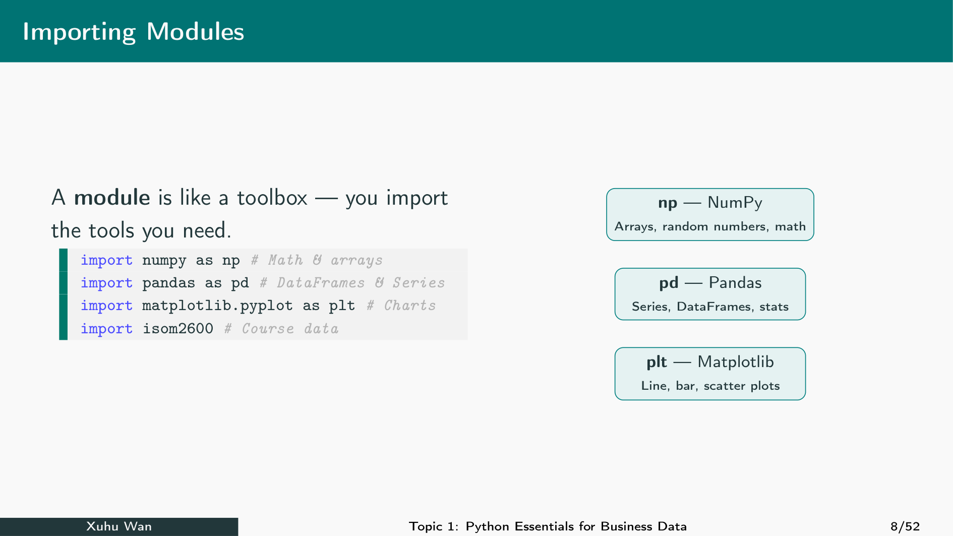
import numpy as np · import pandas as pd · import matplotlib.pyplot as plt · from scipy import stats
Wildcard Imports and Common Errors
from math import * is another form. It brings many public names into the session. Prefer explicit imports so the source of each name is clear.
Wildcard imports can hide existing names. Advanced import mechanisms are outside this chapter.
| Error | Check |
|---|---|
ModuleNotFoundError |
Package spelling and current environment |
NameError: np is not defined |
Whether import numpy as np ran |
AttributeError |
Function spelling; overwritten module name |
They make names traceable and reduce accidental name collisions.
Sources: Python modules
Worked check: Match the import
Calculate the square root of 144 in two ways: with a module prefix and with a directly imported function.
Both results are 12.0. The available calling name follows the import statement.
NumPy Arrays
Question: How do arrays calculate on many observations?
Result: Create arrays, inspect their structure and explain element-wise results.
Use the import rules from 0.5.1 to give numerical tools the name np.
Create a NumPy Array
NumPy provides arrays for numerical calculations. np.array(...) converts a list into an array. Import NumPy before using np.
An ndarray stores a structured collection of values. This array is one-dimensional. Its printed form usually omits commas.
A NumPy array with those three values.
Sources: NumPy arrays
List Multiplication versus Array Multiplication
A list multiplied by 2 repeats its items. An array multiplied by 2 doubles each numerical value.
The list repeats; the array multiplies element by element.
Array Multiplication: The Picture
The list repeats the sequence; the array produces one doubled value per original item. Repetition is valid list behaviour, but does not calculate doubled prices.
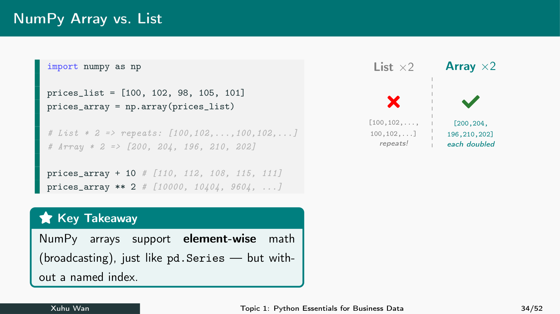
Array Attributes and Methods
An array is an object: it stores values and provides information and tools. The dot in prices.member accesses something belonging to prices.
| Kind | Meaning | Example |
|---|---|---|
| Attribute | Information about the object; read without () |
prices.dtype |
| Method | A function belonging to the object; call with () |
prices.sum() |
The attribute shape reports dimensions: (3,) means three items in one dimension. size reports the total number of items. dtype reports the shared stored value type; dtype=float requests decimal storage. The outer print() is a separate function used to display each result. sum() and max() calculate results without changing prices.
Predict, then try: which expressions use ()? Change prices.sum() to prices.mean() and run again. The method now calculates the average price.
Read information without parentheses, such as prices.dtype. Call a method with parentheses, such as prices.sum(). shape describes dimensions; dtype describes the element type.
Calculate Revenue Element by Element
For equally shaped arrays, corresponding positions are combined. Each position represents one dish category: Wonton, Char Siu and Veggie. Customer count × average bill gives that category’s daily revenue.
Units: customers/day × HK$/customer = HK$/day. The entries must refer to the same dishes in the same order; the total is HK$13,870/day.
A Scalar Applies to Every Element
A scalar is one value. Applying it to every array item is a simple form of broadcasting. Use it for price adjustments and percentage changes.
** raises each item to a power. Other broadcasting cases require compatible shapes; arbitrary array sizes cannot always be combined.
A 10 percent increase in each price.
Conditions Create a Boolean Mask
A comparison returns one True/False result per item. Use the mask to select matching values. Its mean is the fraction of True values.
Two of four prices pass: 0.5, or 50%.
True counts as 1 and False as 0 in numerical aggregation.
Array Summary Statistics
Use sum, mean, median, min, and max to summarise observations. Interpret the units: a mean is not a guarantee about every observation.
The mean is 101.2 customers/day. Observed counts range from 98 to 105. Level and variability answer different questions.
customers.mean() is an array method. np.median(customers) calls a function from NumPy with the array as its argument. The mean is the total divided by the count; the median is the middle of the ordered values.
Standard Deviation: Choose the Denominator
Standard deviation measures spread in the original units. NumPy defaults to ddof=0: variance divides by n. The usual sample standard deviation uses ddof=1: variance divides by n−1.
Outputs: 2.315 and 2.588 customers. Match the convention to the question; pandas defaults to ddof=1.
Variance uses n−1 in its denominator; standard deviation is its square root.
Sources: NumPy std
Random Numbers: A Reproducible Simulation
A simulation creates artificial data. A normal model is a bell-shaped distribution described by its mean and standard deviation. np.random.normal draws numbers from a normal model: loc=28 sets the mean to 28 minutes, scale=6 sets the standard deviation to 6 minutes, and size=5 asks for five numbers.
Keep the seed line when comparing runs; print the simulated values directly.
These are simulated delivery times, not observations. The np.random.seed(42) line makes the example repeatable; 42 is an arbitrary seed. Change size=5 to size=10 and run again to generate ten values. Part 0.5.3 explains the normal model.
Worked check: A price increase
Increase all three prices by 10%, then select the updated prices above HK$50.
The updated prices are 46.2, 63.8 and 30.8; only 63.8 exceeds 50.
SciPy Probability
Question: How does a probability model answer a business question?
Result: Read CDF, PPF and density outputs with units and stated assumptions.
Arrays summarise observed values; a probability model calculates what follows from assumptions.
SciPy: A Normal Probability Model
scipy.stats supplies probability distributions. A normal distribution is a bell-shaped model described by a mean and standard deviation. Its use is an assumption about the data. Here, loc=8 sets the mean to 8 minutes and scale=2 sets the standard deviation to 2 minutes. The methods model.mean() and model.std() report these chosen parameters.
loc is the mean μ and scale is the standard deviation σ, not the variance. Times here are measured in minutes. A normal model allows negative values, so its suitability for time data must be checked.
Standard deviation 2, not variance 2.
Sources: SciPy normal distribution
CDF: A Value Gives a Probability
CDF means cumulative distribution function: P(X ≤ x). For the normal model with mean 8 and standard deviation 2, what fraction of waiting times is at most 10 minutes?
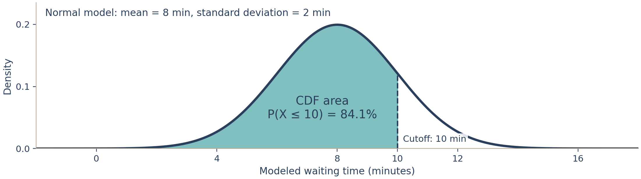
About 84.1% lie at or below 10 minutes under this model. For a continuous normal distribution, < and ≤ give the same probability.
A cutoff value goes in; a probability comes out.
Upper Tail: Exceeding a Limit
For the same normal model (mean 8, standard deviation 2), shade the area to the right of 10 minutes: P(X > 10). The total area is 1, so subtract the CDF’s left-hand area from 1.
For extreme tails, SciPy’s sf (survival function) is numerically preferable to subtraction. This chapter first uses 1 − CDF to make the probability reasoning explicit.
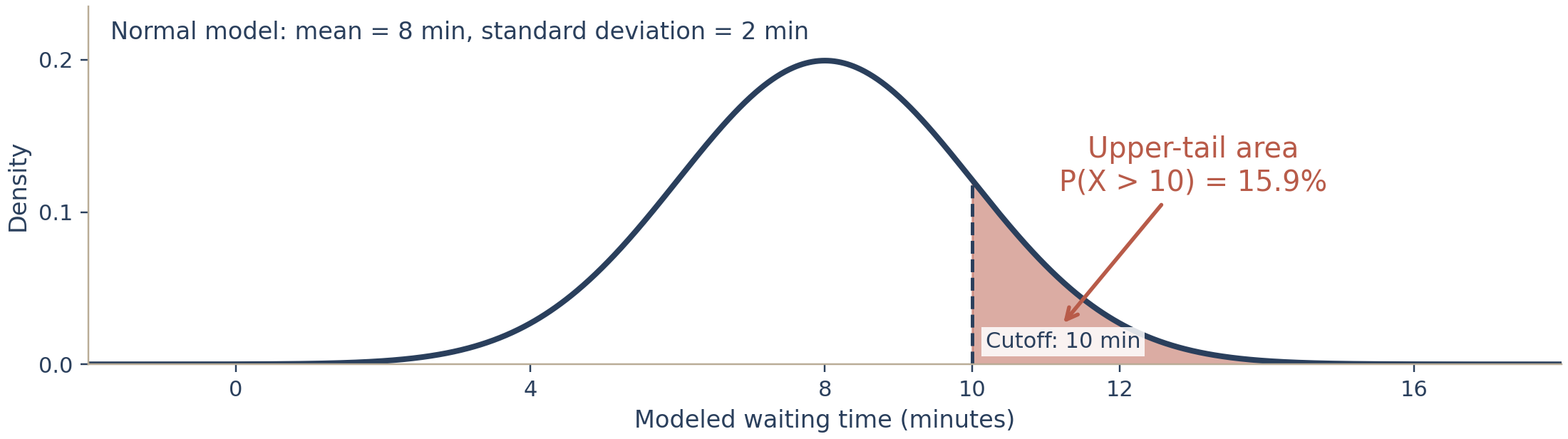
The shaded upper tail is about 15.9%. The two areas sum to 100%: 84.1% + 15.9%.
Probability Between Two Values
To find the probability between 6 and 10 minutes, subtract the cumulative probability up to 6 from the cumulative probability up to 10.
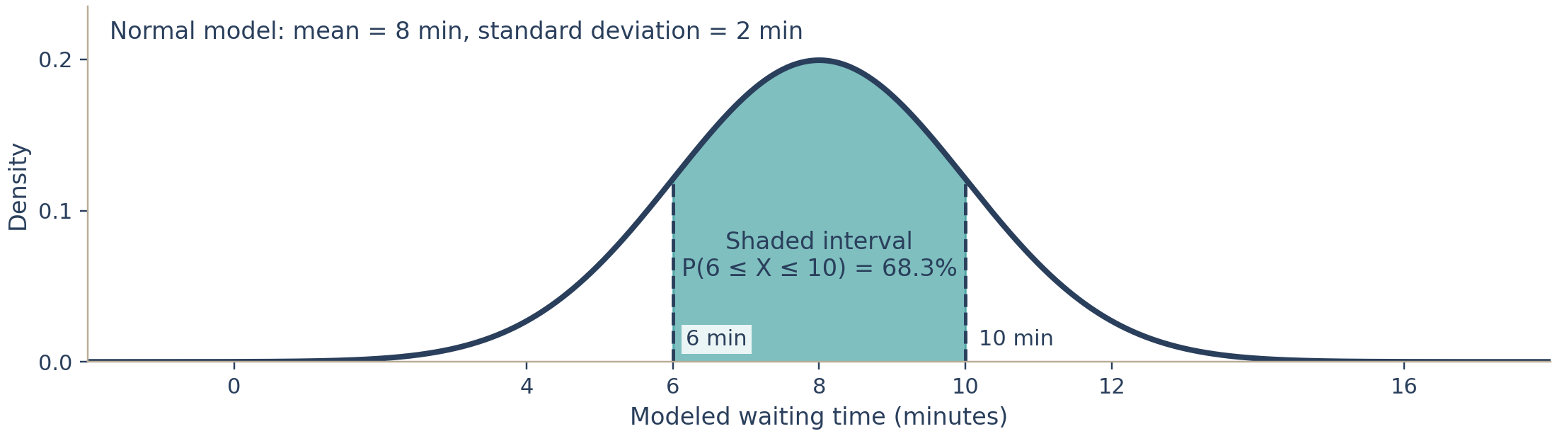
The probability is about 68.3%, matching the normal interval within one standard deviation of its mean.
CDF(b) − CDF(a), for a < b.
PPF: A Probability Gives a Value
PPF means percent point function, the inverse CDF: probability → cutoff. Start with a shaded left-tail area of 5% and find the cutoff x. Here the normal model has mean 8 and standard deviation 2.
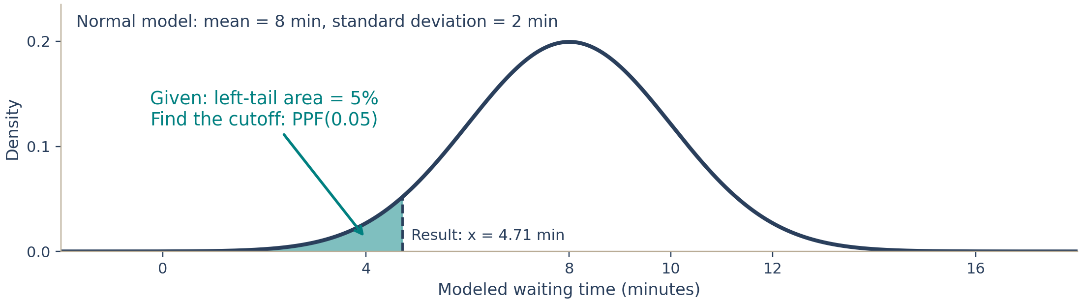
About 5% of modelled waiting times are at or below 4.71 minutes. Use 0.05, not 5.
A probability between 0 and 1 goes in; a cutoff in the original units comes out.
Delivery-Time Service Target
A service-level agreement (SLA) is a promised service standard. Assume delivery times follow a normal model with mean 28 and standard deviation 6 minutes. How often is a 40-minute limit exceeded?
The model assumes the same distribution applies to these deliveries. Traffic, extreme delays, or different routes may invalidate it. The percentile does not guarantee every order arrives in that time.
About 2.28% exceed 40 minutes; the modelled 95th percentile is 37.87 minutes. These are model estimates, not observed frequencies.
PDF: Density Is Not Probability
PDF is probability density, the height of a continuous distribution’s curve. Probability is area over an interval, not the height at a point.
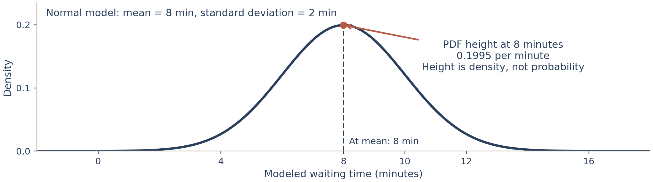
The density is about 0.1995 per minute; the cumulative probability is 0.5. They measure different things.
No. It gives density; interval probability is an area.
Worked check: A 90% delivery target
For a normal model with mean 28 and standard deviation 6 minutes, find the 90th percentile. Pass it back into CDF to check the probability.
About 35.69 minutes is the model’s 90th percentile; CDF returns 0.90. This is a model-based service target, not a guarantee for every order.
Chapter Wrap-up
Chapter 0 and its companion chapter prepare Week 1’s ungraded, in-class Retail Inventory Review. Read the assigned material and bring a compact note; the practice examples are learning aids, not a take-home assignment. Use the student Course Plan PDF for the classroom sequence and the supplied notebook for group work. Consult the current course outline for assessment weights and participation arrangements.
You can now read a line of Python and say, before running it, what it will print. Specifically, you can tell / from // and know that the first always produces a float and the second floors toward minus infinity; you know that 0.1 + 0.2 is not 0.3 and compare floats with a tolerance; you know that True is 1 and that sum(condition) counts. You can slice any sequence with the start-inclusive, stop-exclusive rule and compute the length of the slice by subtraction, and you know that range obeys the same rule. You hold the names-and-objects model: assignment attaches a label, mutation changes the object, and so b = a followed by a change to b alters a for a list and not for an integer — with .copy() when you want independence and is reserved for None. You can choose a tuple for a fixed record, a set for membership and de-duplication, and a dictionary for a lookup, and you know when a missing name should raise and when it should default. You can write a branch whose thresholds are ordered strictest-first, a loop that uses enumerate rather than an index, break to stop and continue to skip, and a comprehension in which you can tell a filter from a label. You can define a function with a docstring, know that it returns None without return, avoid the mutable default, accept *args and **kwargs, pass a lambda as a key=, keep state out of globals, format a number with :.2f, :.2% and :,, and catch the specific exception you expect.
You can also distinguish installation from import, use NumPy for calculations on ordered values, and read a SciPy result as a probability, a cutoff or a density. State the model assumptions before interpreting a service target.
Chapter 1 builds on this foundation with business-data examples. Keep asking the same questions: what object does this name refer to, which items does this slice select, what does this function return, and does this method change the original object or return a new value? Those checks help you explain the output before drawing a conclusion.
The companion slide deck for this chapter (Chapter 0 in the course slides) follows the same five sections with the same examples, and adds multiple-choice questions on each trap and “your turn” practice cells — FizzBuzz, clean_and_count, the top-three words — that check your answer automatically. Work through them before the Chapter 1 lecture; the ones you get wrong are the ones to revisit here.
Further reading
The Python tutorial explains expressions, strings and positional slices. The functions tutorial explains argument binding and return values.